Data analysis
Contents
1. Downloading the data
Here we assume you download a small part of the MAXI archive data. Change directory to your chosen working directory; suppose it is $HOME/analysis/ Then, run the script mxdownload_wget, specifying the coordinates (in J2000) of the center of your chosen region, radius (optional), the observation period, and instruments/modes (optional). The MAXI archive data is available since 2009-08-15 (MJD=55058).The format of mxdownload_wget is,
mxdownload_wget -coordinates RA,DEC -date_from TSTART -date_to TSTOP (YYYY-MM-DD or MJD) [and OPTIONS]
The following is an example; it downloads the MAXI data from DARTS for the area centered at the Crab Nebula observed from 2010-01-01 and 2010-01-31.
 cd $HOME/analysis/
 mxdownload_wget --coordinates 83.633083,22.0145 -date_from 2010-01-01 -date_to 2010-01-31 -uri https://darts.isas.jaxa.jp/pub/maxi/mxdata/
All the MAXI data that satisfy the specified conditions are downloaded from DARTS to the new "obs" sub-directory under the current directory. If you omit the "-uri" option, the data are downloaded from HEASARC.
MAXI does not monitor all the 768 sky regions everyday, some data of some regions for some days are not available. Also, There is a lack of data for different reasons: MAXI shutdown, downlink problems, processing errors etc. The detailed information about those problems will be appeared on the MAXI home page.
Users can specify a radius and an instrument mode with options, -radius (default: 8.0 deg) and -instruments (default: gsc_low), respectively. The following is an example of downloading the SSC data for the radius of 10 degrees.
mxdownload_wget -coordinates 10.00,-20.000 -dates 2010-01-01,2010-01-31 -radius 10 -instruments ssc_med -uri https://darts.isas.jaxa.jp/pub/maxi/mxdata/
You can view a concise on-line help by fhelp mxdownload_wget. The two options -dryrun and -planonly are for dry-running (simulated run) and can be useful to see how it works and how many data files will be (attempted to be) downloaded.
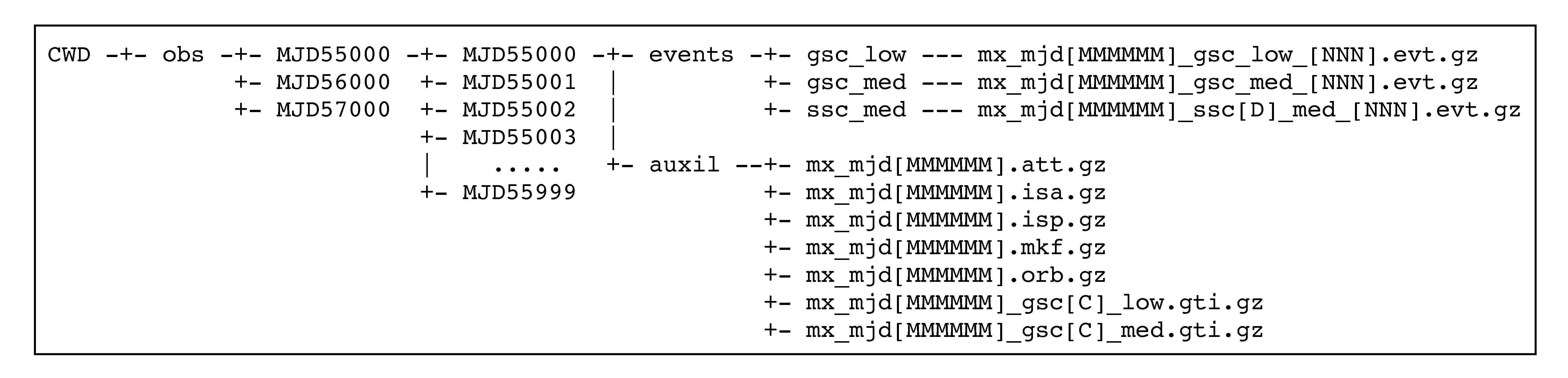
The following is the directory structure created by mxdownload_wget
and the following is the file/directory structure after the pipe-line processing by mxproduct explained in detail in the next section:
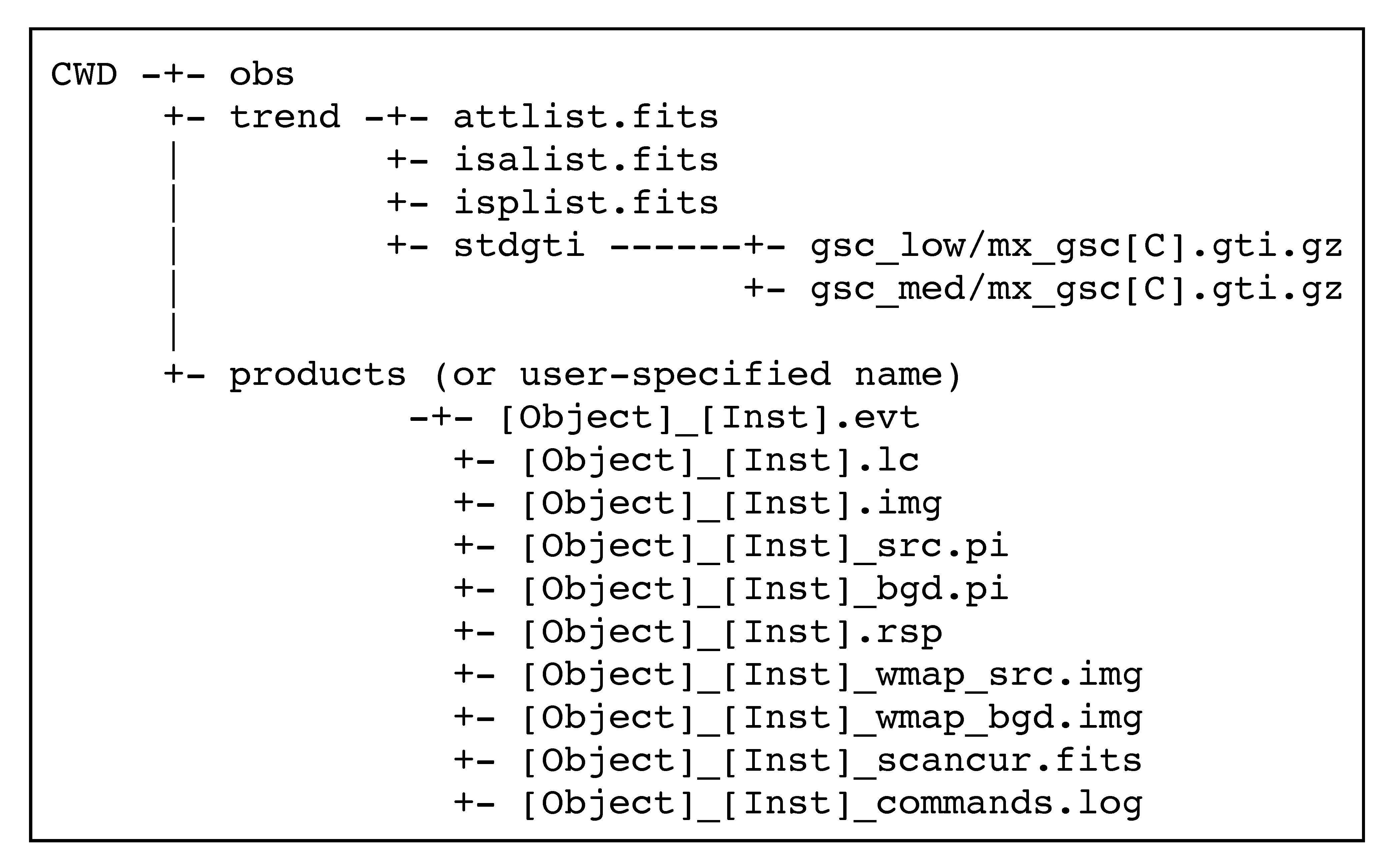
where CWD refers to the current working-directory, (gsc_low, gsc_med, ssc_med) is the instrument_mode (data rate), [MMMMM] is the Modified Julian Day (MJD) in 5 digits, [C] is the counter-ID of the GSC (0, 1, 2, 3, 4, 5, 6, 7, 8, 9, a, b), [D] is the detector-ID of the SSC (“h” or “z”), [NNN] is the “Healpix”-ID, as explained below, [Object] is the prefix specified by a user (object option of mxproduct), and [Inst] is one of (g_low, g_med, s_med), corresponding to (gsc_low, gsc_med, ssc_med), respectively.
Healpix is the library to define the regions on the sky, dividing the entire sky into regions with a similar area-size to one another. The data in the MAXI archive make use of Healpix system with NSIDE=8, RING format, which divides the entire sky into 768 regions. The J2000 celestial coordinates (RA, DEC) that MAXI uses are related to the Healpix coordinates (θ, φ) for each pixel-ID with the following formula:
(RA, DEC) = (φ, π/2 - θ) [radian] (J2000).
2. Analyzing the data
Now you have the raw MAXI data in your local disk, you are ready to make data reduction, using one of MAXI FTOOLS, mxproduct, to get the spectra and light-curve with your choice of filtering selections.
2.1. Data reduction by mxproduct
Introduction
The following is the simplest example of the data reduction of the GSC-low data of Crab to make the spectra and light-curves. In this example, mxproduct is run at the root data-directory, which contains the directory obs/ .
mxproduct 83.633083 22.014500 2010-01-01 2010-01-31 object=crab
This will create the GSC science products of spectra for the default region, response file for them, and light-curves in the default energy band, all for the region around the coordinates of (RA, DEC) [J2000] for the period between TSTART and TSTOP. The science product files are stored in the directory ./products/ (or, user-specified name by the option, outpath), which is created if it does not exist.
The ftool help is given by
fhelp mxproduct
or read through this document for the complete reference.
Overview
The format of mxproduct is,
mxproduct RA Dec TSTART TSTOP [OPTIONS]
mxproduct requires 4 mandatory parameters; the center coordinates (RA and Dec) and the start and end time. RA and Dec should be given in degree (J2000). The format of TSTART and TSTOP is either YYYY-MM-DD or YYYY-MM-DDThh:mm:ss, where YY, MM, DD, hh, mm, ss are year, month, day, hour, minute and second, respectively. When only YYYY-MM-DD is specified, TSTART is identical to YYYY-MM-DDT00:00:00 and TSTOP is identical to YYYY-MM-DDT23:59:59.
In addition, mxproduct accepts several optional arguments, each of which is given in the format of option=PARAMETER.
- Instrument/Mode
- Spatial filter
- Energy-band filter.
Here is the detail of how to specify optional parameters.
- Instrument/Mode
- The GSC has 2 data types: gsc_low and gsc_med. Users must choose either of them. Our recommendation is gsc_low, which is the default. In case to choose the medium data, set the option gscdl=med.
- Spatial filter (Region files, recommended)
- You can supply the source and the background region files for GSC and/or SSC. See the options srcregfile_gsc, bgdregfile_gsc, srcregfile_ssc, bgdregfile_ssc. mxproduct runs without region files, in which case the background region is automatically chosen before and after the scan of the source. However, it is reported that the estimated background level is underestimated when region files are not specified. Thus, we recommend specifying the source and background region files.
- The region-file format is the ds9 format in plain text with the fk5 coordinate system in degrees. When saving a region file in ds9, be careful to select coordinates in degrees (sexagesimal may be selected by default in ds9). Currently, acceptable shape of the source region is a simple "circle", and the background region is "circle - circle". The background region has to be within a radius of 8.0 deg from the center coordinates, which can be changed by adding an option, radi_o. See the examples.
- Example for the source region file:
- Example for the background region file, which is a "ring" surrounding the source region:
- Energy-band filter
- In mxproduct, multi-band light-curves are generated and stored in multiple extensions in a single output FITS file.
- The default energy bands are 2.0–5.95 and 6.0–11.95 keV for GSC, 0.7–1.997 and 2.000–6.997 keV for SSC.
- If you want to change the energy bands, you can supply a plain text file that describes your desired (multiple) energy bands. See the options ebandfname_gsc,ebandfname_ssc.
- Each line of the file consists of a pair (Minimum, Maximum) of the energy in keV, separated by a single space.
- The following is an example for specifying three energy bands, 2–5.95, 6–11.95, and 12–20 keV.
-
2.0 5.95 6.0 11.95 12.0 20.0
 # Region file format: DS9 version 4.1
 global color=green dashlist=8 3 width=1 font="helvetica 10 normal roman" select=1 highlite=1 dash=0 fixed=0 edit=1 move=1 delete=1 include=1 source=1
 fk5
 circle(49.951,41.512,6000")
 # Region file format: DS9 version 4.1
 global color=green dashlist=8 3 width=1 font="helvetica 10 normal roman" select=1 highlite=1 dash=0 fixed=0 edit=1 move=1 delete=1 include=1 source=1
 fk5
 circle(49.951,41.512,108000")
 -circle(49.951,41.512,7200")
Output files
mxproduct generates the GSC and/or SSC science products
(spectra, spectral response file, and light-curves)
in the directory products/ (or, user can specify the name by the command-line option, "outpath") , as well as some auxiliary files
in the directory trend/, both in the current directory.
The default energy bands are 2.0–5.95 and 6.0–11.95 keV for the GSC, 0.7–1.997 and 2.000–6.997 keV for the SSC.
The following is a set of example product filenames for GSC_Low, where the command-line option of object=crab is given.
For GSC_Med and SSC_Med, replace g_low
with g_med
and s_med
, respectively.
- Event file
- crab_g_low.evt
- Images
- crab_g_low.img
crab_g_low_wmap_src.img
crab_g_low_wmap_bgd.img - Spectra and responses
- crab_g_low_src.pi
crab_g_low_bgd.pi
crab_g_low.rsp - Light-curves
- crab_g_low.lc
- Scancur file (observation condition for the target)
- crab_g_low_scancur.fits
- Command log
- mxproduct.log (created at the path you ran mxproduct)
During the processing, many intermediate files (such as, GTI files, spectrum files for individual cameras) are created in the same products (or user-specified name) directory. They are automatically left after the processing in default, unless cleanup=yes is specified. The diagram in the previous subsection summarizes the directory and file structure.
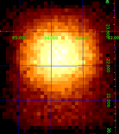
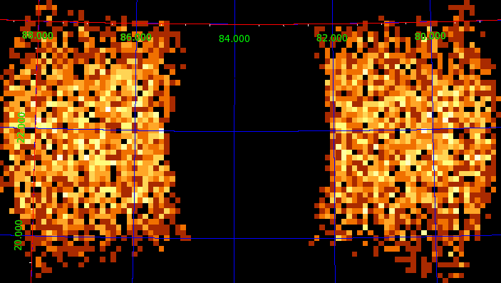
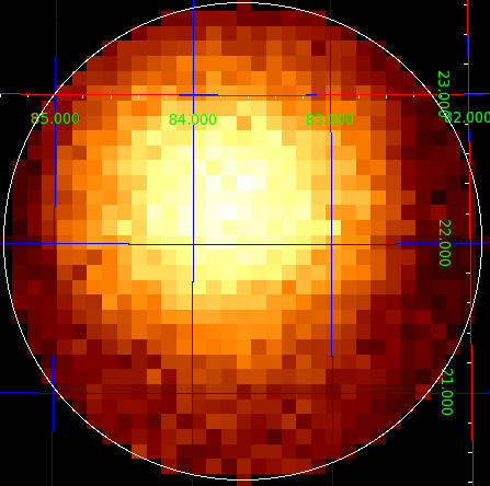
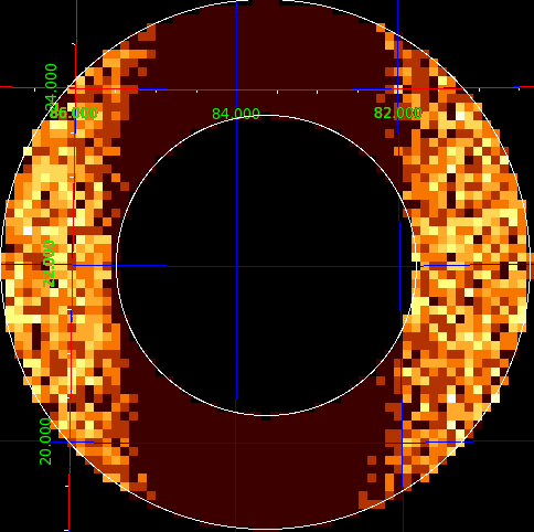
The following figures show examples of WMAP image of Crab for source and background regions without (default settings) and with the region files. Without region files, the default source and background data are selected by elongation angles from the target in a scan direction and in a direction perpendicular to the scan direction. The generated images are neither exposure-corrected nor background-subtracted.
Options
Examples
- The simplest form for the source1 at (RA, DEC)=(350°, −10°).
mxproduct object=src1 350 -10 2010-01-01 2010-01-31 - Processing the data for the radius of 10 degrees of Crab Nebura, where the MAXI data directory obs/ is mounted in /My/Data/Maxi/.
mxproduct object=crab mountdata=1 datapath=/My/Data/Maxi radi_o=10 83.633083 22.014500 2010-01-01 2010-01-31 - Specifying region files for source and background.
mxproduct object=crab srcregfile_gsc=src.reg bgdregfile_gsc=bgd.reg 83.633083 22.014500 2010-01-01 2010-01-31 - Specifying energy bands for GSC light-curves in a text file, gsc_eband.list, a directory name for output files, test1/, and start/stop time with hh:mm:ss.
mxproduct object=crab ebandfname_gsc=gsc_eband.list outpath=test1 83.633083 22.014500 2010-01-01T08:00:00 2010-01-31T20:00:00 - Example of the SSC data processing.
mxproduct object=crab skip_gsc=1 skip_ssc=0 83.633083 22.014500 2010-01-01 2010-01-31
2.2. Data analysis examples
Width of the spectral bin is 50 eV for GSC, and 3.65 eV for SSC.
2.2.1. Spectral analysis
The spectra and response files generated by mxproduct are in the standard FITS format. You can use your favorite software to analyze them. The following is the standard entry-level procedure with the XANADU/HEAsoft spectral-analysis package XSPEC to view the background-subtracted spectrum.
 xspec

 cpd /xw
 data 1:1 "crab_g_low_src.pi"
 back 1   "crab_g_low_bgd.pi"
 resp 1   "crab_g_low.rsp"
 setplot energy
 ignore bad

 iplot ldata

 log x on 1
 log y on 1
 label t Crab
 lwidth 5
 rescale x 1 10
 plot
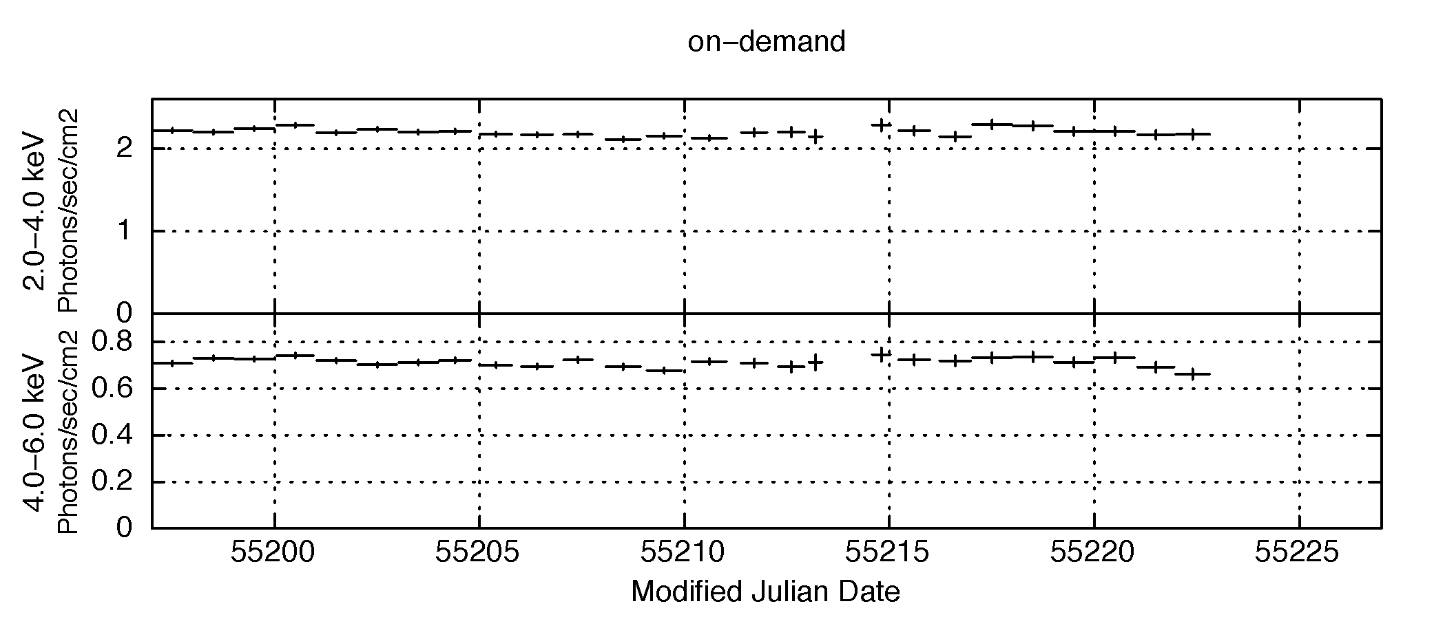
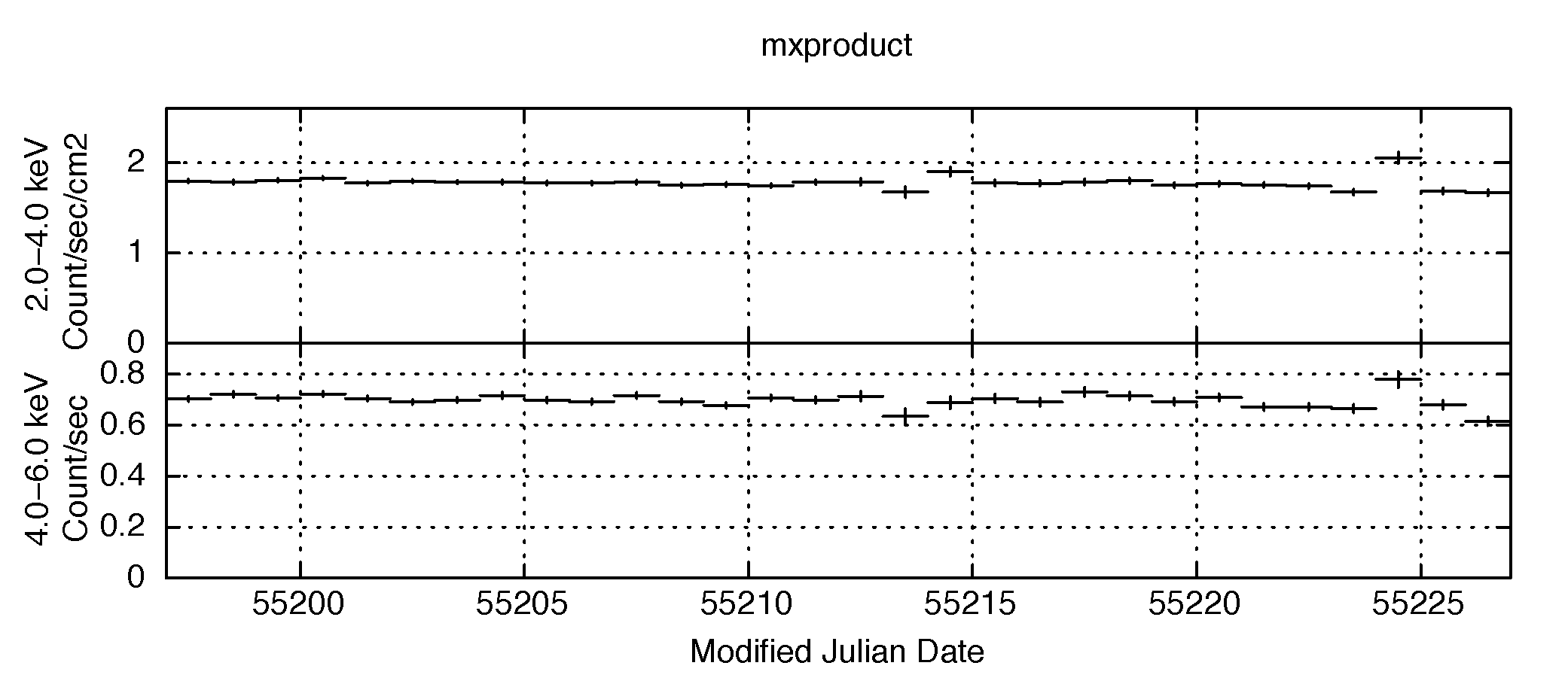
2.2.2. Time-series analysis
The generated FITS file of the light-curves
(crab_g_low.lc in the example above)
contains the same number of the FITS extensions as that of
the energy bands specified in the input text file
(gsc_eband.list in the example above)
with the
ebandfname_gsc
(or ebandfname_ssc) option.
Each FITS Extension is named LCDAT_PIBANDn for the (n+1)-th line of the energy band in the input gsc_eband.list.
For example, the FITS Extension LCDAT_PIBAND0 contains the light-curve for the energy-band of the first line in gsc_eband.list.
Each bin-width of a light-curve is 40~200 sec, which corresponds to the period of a single MAXI scan in which
the source is in the field-of-view. The light-curve bins are separated by the intervals between the two
successional scans, which are ~92 min (= ISS orbital period) in most cases but can be as short as ~15 min.
You can plot the light curve(s) with your favorite software, specifying the TIME as X-axis, and the RATE and RERR columns as Y-axis and its error, respectively. The following is the example with the general plotting tool LCURVE in HEAsoft:
lcurve nser=1 cfile1="products/crab_g_low.lc" window="-" dtnb=INDEF nbint=INDEF outfile=" " plot=yes plotdev="/xw"
Go to Tips, Tricks, and Traps for more details.